nIXS $M_{4,5}$
Inelastic x-ray scattering IXS (non-resonant) nIXS or x-ray Raman scattering allows one to measure non-dipolar allowed transitions. A powerful technique to look at even $d$-$d$ transitions with well defined selection rules \cite{Haverkort:2007bv, vanVeenendaal:2008kv, Hiraoka:2011cq}, but can also be used to determine orbital occupations of rare-earth ions that are fundamentally not possible to determine using dipolar spectroscopy \cite{Willers:2012bz}.
This tutorial compares calculated spectra to experiment. In order to make the plots you need to download the experimental data. You can download them in a zip file here nio_data.zip. Please unpack this file and make sure to have the folders NiO_Experiment and NiO_Radial in the same folder as you do the calculations. And as always, if used in a publication, please cite the original papers that published the data.
The first example shows low energy $d$-$d$ transitions in NiO. The input is:
- NIXS_dd.Quanty
-- This example calculates the d-d excitations in NiO using non-resonant Inelastic X-ray
-- Scattering. This is one of the most beautiful spectroscopy techniques as the selection
-- rules are very "simple" and straight forward.

-- We use the A^2 term of the interaction to make transitions between states with photons
-- of much higher energy. These photons now cary non negligible momentum and one can make
-- transitions beyond the dipole limit.

-- Here we look at k=2 and k=4 transitions between the Ni 3d orbitals

-- We use the definitions of all operators and basis orbitals as defined in the file
-- include and can afterwards directly continue by creating the Hamiltonian
-- and calculating the spectra

dofile("Include.Quanty")

-- The parameters and scheme needed only includes the ground-state (d^8) configuration

-- We follow the energy definitions as introduced in the group of G.A. Sawatzky (Groningen)
-- J. Zaanen, G.A. Sawatzky, and J.W. Allen PRL 55, 418 (1985)
-- for parameters of specific materials see
-- A.E. Bockquet et al. PRB 55, 1161 (1996)
-- After some initial discussion the energies U and Delta refer to the center of a configuration
-- The L^10 d^n   configuration has an energy 0
-- The L^9  d^n+1 configuration has an energy Delta
-- The L^8  d^n+2 configuration has an energy 2*Delta+Udd
--
-- If we relate this to the onsite energy of the L and d orbitals we find
-- 10 eL +  n    ed + n(n-1)     U/2 == 0
--  9 eL + (n+1) ed + (n+1)n     U/2 == Delta
--  8 eL + (n+2) ed + (n+1)(n+2) U/2 == 2*Delta+U
-- 3 equations with 2 unknowns, but with interdependence yield:
-- ed = (10*Delta-nd*(19+nd)*U/2)/(10+nd)
-- eL = nd*((1+nd)*Udd/2-Delta)/(10+nd)
--
-- note that ed-ep = Delta - nd * U and not Delta
-- note furthermore that ep and ed here are defined for the onsite energy if the system had
-- locally nd electrons in the d-shell. In DFT or Hartree Fock the d occupation is in the end not
-- nd and thus the onsite energy of the Kohn-Sham orbitals is not equal to ep and ed in model
-- calculations.
--
-- note furthermore that ep and eL actually should be different for most systems. We happily ignore this fact
--
-- We normally take U and Delta as experimentally determined parameters

-- number of electrons (formal valence)
nd = 8
-- parameters from experiment (core level PES)
Udd     =  7.3
Delta   =  4.7
-- parameters obtained from DFT (PRB 85, 165113 (2012))
F2dd    = 11.14
F4dd    =  6.87
F2pd    =  6.67
tenDq   =  0.56
tenDqL  =  1.44
Veg     =  2.06
Vt2g    =  1.21
zeta_3d =  0.081
Bz      =  0.000001
H112    =  0.120

ed      = (10*Delta-nd*(19+nd)*Udd/2)/(10+nd)
eL      = nd*((1+nd)*Udd/2-Delta)/(10+nd)

F0dd    = Udd + (F2dd+F4dd) * 2/63

Hamiltonian =  F0dd*OppF0_3d + F2dd*OppF2_3d + F4dd*OppF4_3d + zeta_3d*Oppldots_3d + Bz*(2*OppSz_3d + OppLz_3d) + H112 * (OppSx_3d+OppSy_3d+2*OppSz_3d)/sqrt(6) + tenDq*OpptenDq_3d + tenDqL*OpptenDq_Ld + Veg * OppVeg + Vt2g * OppVt2g + ed * OppN_3d + eL * OppN_Ld

-- we now can create the lowest Npsi eigenstates:
Npsi=3
-- in order to make sure we have a filling of 8 electrons we need to define some restrictions
StartRestrictions = {NF, NB, {"000000 00 1111111111 0000000000",8,8}, {"111111 11 0000000000 1111111111",18,18}}

psiList = Eigensystem(Hamiltonian, StartRestrictions, Npsi)
oppList={Hamiltonian, OppSsqr, OppLsqr, OppJsqr, OppSx_3d, OppLx_3d, OppSy_3d, OppLy_3d, OppSz_3d, OppLz_3d, Oppldots_3d, OppF2_3d, OppF4_3d, OppNeg_3d, OppNt2g_3d, OppNeg_Ld, OppNt2g_Ld, OppN_3d}

-- print of some expectation values
print("  #    <E>      <S^2>    <L^2>    <J^2>    <S_x^3d> <L_x^3d> <S_y^3d> <L_y^3d> <S_z^3d> <L_z^3d> <l.s>    <F[2]>   <F[4]>   <Neg^3d> <Nt2g^3d><Neg^Ld> <Nt2g^Ld><N^3d>");
for i = 1,#psiList do
  io.write(string.format("%3i ",i))
  for j = 1,#oppList do
    expectationvalue = Chop(psiList[i]*oppList[j]*psiList[i])
    io.write(string.format("%8.3f ",expectationvalue))
  end
  io.write("\n")
end


-- in order to calculate nIXS we need to determine the intensity ratio for the different multipole intensities
-- ( see PRL 99, 257401 (2007) for the formalism )
-- in short the A^2 interaction is expanded on spherical harmonics and Bessel functions
-- The 3d Wannier functions are expanded on spherical harmonics and a radial wave function
-- For the radial wave-function we calculate <R(r) | j_k(q r) | R(r)>
-- which defines the transition strength for the multipole of order k

-- The radial functions here are calculated for a Ni 2+ atom and stored in the folder NiO_Radial
-- more sophisticated methods can be used

-- read the radial wave functions
-- order of functions
-- r	1S	2S	2P	3S	3P	3D
file = io.open( "NiO_Radial/RnlNi_Atomic_Hartree_Fock", "r")
Rnl = {}
for line in file:lines() do
  RnlLine={}
  for i in string.gmatch(line, "%S+") do
    table.insert(RnlLine,i)
  end
  table.insert(Rnl,RnlLine)
end

-- some constants
a0      =  0.52917721092
Rydberg = 13.60569253
Hartree = 2*Rydberg

-- dd transitions from 3d (index 7 in Rnl) to 3d (index 7 in Rnl)
-- <R(r) | j_k(q r) | R(r)>
function RjRdd (q)
  Rj0R = 0
  Rj2R = 0
  Rj4R = 0
  dr = Rnl[3][1]-Rnl[2][1]
  r0 = Rnl[2][1]-2*dr
  for ir = 2, #Rnl, 1 do
    r = r0 + ir * dr
    Rj0R = Rj0R + Rnl[ir][7] * SphericalBesselJ(0,q*r) * Rnl[ir][7] * dr
    Rj2R = Rj2R + Rnl[ir][7] * SphericalBesselJ(2,q*r) * Rnl[ir][7] * dr
    Rj4R = Rj4R + Rnl[ir][7] * SphericalBesselJ(4,q*r) * Rnl[ir][7] * dr
  end
  return Rj0R, Rj2R, Rj4R
end

-- the angular part is given as C(theta_q, phi_q)^* C(theta_r, phi_r)
-- which is a potential expanded on spherical harmonics
function ExpandOnClm(k,theta,phi,scale)
  ret={}
  for m=-k, k, 1 do
    table.insert(ret,{k,m,scale * SphericalHarmonicC(k,m,theta,phi)})
  end
  return ret
end

-- define nIXS transition operators
function TnIXS_dd(q, theta, phi)
  Rj0R, Rj2R, Rj4R = RjRdd(q)
  k=0
  A0 = ExpandOnClm(k, theta, phi, I^k*(2*k+1)*Rj0R)
  T0 = NewOperator("CF", NF, IndexUp_3d, IndexDn_3d, A0)
  k=2
  A2 = ExpandOnClm(k, theta, phi, I^k*(2*k+1)*Rj2R)
  T2 = NewOperator("CF", NF, IndexUp_3d, IndexDn_3d, A2)
  k=4
  A4 = ExpandOnClm(k, theta, phi, I^k*(2*k+1)*Rj4R)
  T4 = NewOperator("CF", NF, IndexUp_3d, IndexDn_3d, A4)
  T = T0+T2+T4
  T.Chop()
  return T
end

-- q in units per a0 (if you want in units per A take 5*a0 to have a q of 5 per A)
q=4.5

print("for q=",q," per a0 (",q / a0," per A) The ratio of k=0, k=2 and k=4 transition strength is:",RjRdd(q))

-- define some transition operators
qtheta=0
qphi=0
Tq001 = TnIXS_dd(q,qtheta,qphi)

qtheta=Pi/2
qphi=Pi/4
Tq110 = TnIXS_dd(q,qtheta,qphi)

qtheta=acos(sqrt(1/3))
qphi=Pi/4
Tq111 = TnIXS_dd(q,qtheta,qphi)

qtheta=acos(sqrt(9/14))
qphi=acos(sqrt(1/5))
Tq123 = TnIXS_dd(q,qtheta,qphi)

-- calculate the spectra
nIXSSpectra = CreateSpectra(Hamiltonian, {Tq001, Tq110, Tq111, Tq123}, psiList, {{"Emin",-1}, {"Emax",6}, {"NE",3000}, {"Gamma",0.1}})

-- print the spectra to a file
nIXSSpectra.Print({{"file","NiOnIXS_dd.dat"}})

-- a gnuplot script to make the plots
gnuplotInput = [[
set autoscale
set xtic auto
set ytic auto
set style line  1 lt 1 lw 1 lc rgb "#FF0000"
set style line  2 lt 1 lw 1 lc rgb "#0000FF"
set style line  3 lt 1 lw 1 lc rgb "#00C000"
set style line  4 lt 1 lw 1 lc rgb "#800080"
set style line  5 lt 1 lw 3 lc rgb "#000000"

set xlabel "E (eV)" font "Times,12"
set ylabel "Intensity (arb. units)" font "Times,12"

set out 'NiOnIXS_dd.ps'
set size 1.0, 0.3
set terminal postscript portrait enhanced color  "Times" 12

set yrange [0:6.5]

plot "NiO_Experiment/NIXS_dd_JSR_16_469_2009" using 1:($2*0.01) title 'experiment' with filledcurves y1=0 ls 5 fs transparent solid 0.5,\
     "NiOnIXS_dd.dat" using 1:(-$15 -$17 -$19 +3.25) title 'q // 111' with lines ls  3,\
     "NiOnIXS_dd.dat" using 1:(-$21 -$23 -$25 +2.50) title 'q // 123' with lines ls  4,\
     "NiOnIXS_dd.dat" using 1:(-$9  -$11 -$13 +1.75) title 'q // 011' with lines ls  2,\
     "NiOnIXS_dd.dat" using 1:(-$3   -$5  -$7 +1.00) title 'q // 001' with lines ls  1
]]

-- write the gnuplot script to a file
file = io.open("NiOnIXS_dd.gnuplot", "w")
file:write(gnuplotInput)
file:close()

-- call gnuplot to execute the script
os.execute("gnuplot NiOnIXS_dd.gnuplot")
-- transform to pdf and eps
os.execute("ps2pdf NiOnIXS_dd.ps  ; ps2eps NiOnIXS_dd.ps  ;  mv NiOnIXS_dd.eps temp.eps  ; eps2eps temp.eps NiOnIXS_dd.eps  ; rm temp.eps")
The spectrum produced:
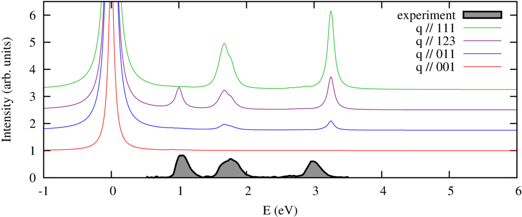 |
| nonresonant inelastic x-ray scattering spectra orientations of the momentum compared to the experimental spectra of a powder. |
|---|
We calculate the spectrum in 4 different directions of momentum transfer. The experimental spectra \cite{Verbeni:2009dx, Huotari:2008kx} are measured on a powder sample and thus do not show the strong momentum direction dependence. In previous \cite{Larson:2007ev} and subsequent \cite{Hiraoka:2009fa} this angular dependence has been observed.
For completeness the output of the script is:
- NIXS_dd.out
  #    <E>      <S^2>    <L^2>    <J^2>    <S_x^3d> <L_x^3d> <S_y^3d> <L_y^3d> <S_z^3d> <L_z^3d> <l.s>    <F[2]>   <F[4]>   <Neg^3d> <Nt2g^3d><Neg^Ld> <Nt2g^Ld><N^3d>
  1   -3.503    1.999   12.000   15.095   -0.370   -0.115   -0.370   -0.115   -0.741   -0.230   -0.305   -1.042   -0.924    2.186    5.990    3.825    6.000    8.175
  2   -3.395    1.999   12.000   15.160   -0.002   -0.000   -0.002   -0.000   -0.003   -0.001   -0.322   -1.043   -0.925    2.189    5.988    3.823    6.000    8.178
  3   -3.286    1.999   12.000   15.211    0.369    0.113    0.369    0.113    0.737    0.227   -0.336   -1.043   -0.925    2.193    5.987    3.820    6.000    8.180
for q=	4.5	 per a0 (	8.5037675605428	 per A) The ratio of k=0, k=2 and k=4 transition strength is:	0.069703673179605	0.1609791731565	0.086144672158063