FY $L_{2,3}M_{4,5}$
The absorption cross section is in principle measured using transmission. Transmission experiments in the soft-x-ray regime can be difficult as the absorption is quite high. Alternatively one can measure the reflectivity, which allows one to retrive the complete conductivity tensor using ellipsometry. As the x-ray wave-length is not large compared to the sample thickness this does not return the average sample absorption, but gives spatial information as well. Known as resonant scattering or reflectometry a beautiful technique, but might be overkill in some situations. A simple but effective way to measure the absorption cross section is to use the total electron yield, which can be measured by grounding the sample via an Ampare meter.
An alternative is to measure the fluorescence yield. Although not proportional to the absorption cross section \cite{Kurian:2012de,vanVeenendaal:1996tb,deGroot:1994tz} an extremely useful technique that contains similar information as absorption. Actually it is often more sensitive to differences in the ground-state and shows more detail in the spectral features. The calculation of fluorescence yield is similar to the calculation of absorption.
In the following example we calculate the excitation of a $2p$ electron into the $3d$ shell of Ni in NiO. ($L_{2,3}$ edge). We integrate over the decay of a $3d$ electron into the $2p$ orbital (removing an electron from the $3d$-shell i.e. $M_{4,5}$) We thus look at the $L_{2,3}$-$M_{4,5}$ FY spectra. (note that one should always list both the excitation as well as the decay channel as the spectra change between different channels).
The input file is:
- FY_L23M45.Quanty
-- This example calculates the fluorescence yield spectra for NiO (L23M45, i.e. 2p to
-- 3d excitation and decay from 3d back to 2p) within the ligand field theory approximation

-- We use the definitions of all operators and basis orbitals as defined in the file
-- 44_50_include and can afterwards directly continue by creating the Hamiltonian
-- and calculating the spectra

dofile("Include.Quanty")

-- The parameters and scheme needed is the same as the one used for XAS

-- We follow the energy definitions as introduced in the group of G.A. Sawatzky (Groningen)
-- J. Zaanen, G.A. Sawatzky, and J.W. Allen PRL 55, 418 (1985)
-- for parameters of specific materials see
-- A.E. Bockquet et al. PRB 55, 1161 (1996)
-- After some initial discussion the energies U and Delta refer to the center of a configuration
-- The L^10 d^n   configuration has an energy 0
-- The L^9  d^n+1 configuration has an energy Delta
-- The L^8  d^n+2 configuration has an energy 2*Delta+Udd
--
-- If we relate this to the onsite energy of the L and d orbitals we find
-- 10 eL +  n    ed + n(n-1)     U/2 == 0
--  9 eL + (n+1) ed + (n+1)n     U/2 == Delta
--  8 eL + (n+2) ed + (n+1)(n+2) U/2 == 2*Delta+U
-- 3 equations with 2 unknowns, but with interdependence yield:
-- ed = (10*Delta-nd*(19+nd)*U/2)/(10+nd)
-- eL = nd*((1+nd)*Udd/2-Delta)/(10+nd)
--
-- For the final state we/they defined
-- The 2p^5 L^10 d^n+1 configuration has an energy 0
-- The 2p^5 L^9  d^n+2 configuration has an energy Delta + Udd - Upd
-- The 2p^5 L^8  d^n+3 configuration has an energy 2*Delta + 3*Udd - 2*Upd
--
-- If we relate this to the onsite energy of the p and d orbitals we find
-- 6 ep + 10 eL +  n    ed + n(n-1)     Udd/2 + 6 n     Upd == 0
-- 6 ep +  9 eL + (n+1) ed + (n+1)n     Udd/2 + 6 (n+1) Upd == Delta
-- 6 ep +  8 eL + (n+2) ed + (n+1)(n+2) Udd/2 + 6 (n+2) Upd == 2*Delta+Udd
-- 5 ep + 10 eL + (n+1) ed + (n+1)(n)   Udd/2 + 5 (n+1) Upd == 0
-- 5 ep +  9 eL + (n+2) ed + (n+2)(n+1) Udd/2 + 5 (n+2) Upd == Delta+Udd-Upd
-- 5 ep +  8 eL + (n+3) ed + (n+3)(n+2) Udd/2 + 5 (n+3) Upd == 2*Delta+3*Udd-2*Upd
-- 6 equations with 3 unknowns, but with interdependence yield:
-- epfinal = (10*Delta + (1+nd)*(nd*Udd/2-(10+nd)*Upd) / (16+nd)
-- edfinal = (10*Delta - nd*(31+nd)*Udd/2-90*Upd) / (16+nd)
-- eLfinal = ((1+nd)*(nd*Udd/2+6*Upd)-(6+nd)*Delta) / (16+nd)
--
--
--
-- note that ed-ep = Delta - nd * U and not Delta
-- note furthermore that ep and ed here are defined for the onsite energy if the system had
-- locally nd electrons in the d-shell. In DFT or Hartree Fock the d occupation is in the end not
-- nd and thus the onsite energy of the Kohn-Sham orbitals is not equal to ep and ed in model
-- calculations.
--
-- note furthermore that ep and eL actually should be different for most systems. We happily ignore this fact
--
-- We normally take U and Delta as experimentally determined parameters

-- number of electrons (formal valence)
nd = 8
-- parameters from experiment (core level PES)
Udd     =  7.3
Upd     =  8.5
Delta   =  4.7
-- parameters obtained from DFT (PRB 85, 165113 (2012))
F2dd    = 11.14
F4dd    =  6.87
F2pd    =  6.67
G1pd    =  4.92
G3pd    =  2.80
tenDq   =  0.56
tenDqL  =  1.44
Veg     =  2.06
Vt2g    =  1.21
zeta_3d =  0.081
zeta_2p = 11.51
Bz      =  0.000001
H112    =  0

ed      = (10*Delta-nd*(19+nd)*Udd/2)/(10+nd)
eL      = nd*((1+nd)*Udd/2-Delta)/(10+nd)

epfinal = (10*Delta + (1+nd)*(nd*Udd/2-(10+nd)*Upd)) / (16+nd)
edfinal = (10*Delta - nd*(31+nd)*Udd/2-90*Upd) / (16+nd)
eLfinal = ((1+nd)*(nd*Udd/2+6*Upd) - (6+nd)*Delta) / (16+nd)

F0dd    = Udd + (F2dd+F4dd) * 2/63
F0pd    = Upd + (1/15)*G1pd + (3/70)*G3pd

Hamiltonian =  F0dd*OppF0_3d + F2dd*OppF2_3d + F4dd*OppF4_3d + zeta_3d*Oppldots_3d + Bz*(2*OppSz_3d + OppLz_3d) + H112 * (OppSx_3d+OppSy_3d+2*OppSz_3d)/sqrt(6) + tenDq*OpptenDq_3d + tenDqL*OpptenDq_Ld + Veg * OppVeg + Vt2g * OppVt2g + ed * OppN_3d + eL * OppN_Ld

XASHamiltonian =  F0dd*OppF0_3d + F2dd*OppF2_3d + F4dd*OppF4_3d + zeta_3d*Oppldots_3d + Bz*(2*OppSz_3d + OppLz_3d)+ H112 * (OppSx_3d+OppSy_3d+2*OppSz_3d)/sqrt(6) + tenDq*OpptenDq_3d + tenDqL*OpptenDq_Ld + Veg * OppVeg + Vt2g * OppVt2g + edfinal * OppN_3d + eLfinal * OppN_Ld + epfinal * OppN_2p + zeta_2p * Oppcldots + F0pd * OppUpdF0 + F2pd * OppUpdF2 + G1pd * OppUpdG1 + G3pd * OppUpdG3

-- we now can create the lowest Npsi eigenstates:
Npsi=3
-- in order to make sure we have a filling of 8 electrons we need to define some restrictions
StartRestrictions = {NF, NB, {"000000 00 1111111111 0000000000",8,8}, {"111111 11 0000000000 1111111111",18,18}}

psiList = Eigensystem(Hamiltonian, StartRestrictions, Npsi)
oppList={Hamiltonian, OppSsqr, OppLsqr, OppJsqr, OppSx_3d, OppLx_3d, OppSy_3d, OppLy_3d, OppSz_3d, OppLz_3d, Oppldots_3d, OppF2_3d, OppF4_3d, OppNeg_3d, OppNt2g_3d, OppNeg_Ld, OppNt2g_Ld, OppN_3d}

-- print of some expectation values
print("  #    <E>      <S^2>    <L^2>    <J^2>    <S_x^3d> <L_x^3d> <S_y^3d> <L_y^3d> <S_z^3d> <L_z^3d> <l.s>    <F[2]>   <F[4]>   <Neg^3d> <Nt2g^3d><Neg^Ld> <Nt2g^Ld><N^3d>");
for i = 1,#psiList do
  io.write(string.format("%3i ",i))
  for j = 1,#oppList do
    expectationvalue = Chop(psiList[i]*oppList[j]*psiList[i])
    io.write(string.format("%8.3f ",expectationvalue))
  end
  io.write("\n")
end

-- We calculate the x-ray absorption spectra for z, right circular and left circular polarized light for the ground-state. (3 spectra in total)
XASSpectra = CreateSpectra(XASHamiltonian, {T2p3dz, T2p3dr, T2p3dl}, psiList, {{"Emin",-10}, {"Emax",20}, {"NE",3500}, {"Gamma",1.0}})
XASSpectra.Print({{"file","FYL23M45_XAS.dat"}});

-- and we calculate the FY spectra
FYSpectra = CreateFluorescenceYield(XASHamiltonian, {T2p3dz, T2p3dr, T2p3dl}, {T3d2px, T3d2py, T3d2pz}, psiList, {{"Emin",-10}, {"Emax",20}, {"NE",3500}, {"Gamma",1.0}});
FYSpectra.Print({{"file","FYL23M45_Spec.dat"}});

-- in order to plot both the XAS and FY spectra we can define a gnuplot script
gnuplotInput = [[
set autoscale
set xtic auto
set ytic auto
set style line  1 lt 1 lw 1 lc rgb "#000000"
set style line  2 lt 1 lw 1 lc rgb "#FF0000"
set style line  3 lt 1 lw 1 lc rgb "#00FF00"
set style line  4 lt 1 lw 1 lc rgb "#0000FF"

set xlabel "E (eV)" font "Times,10"
set ylabel "Intensity (arb. units)" font "Times,10"

set out 'FYL23M45.ps'
set terminal postscript portrait enhanced color  "Times" 8 size 7.5,6
set yrange [0:0.6]

set multiplot layout 3, 3

plot "FYL23M45_XAS.dat"  u 1:(-$3 )  title 'z-polarized Sz=-1' with filledcurves y1=0 ls  1 fs transparent solid 0.5,\
     "FYL23M45_Spec.dat" u 1:(4*$2)  title 'FY - x out' with lines ls 2,\
     "FYL23M45_Spec.dat" u 1:(4*$4)  title 'FY - y out' with lines ls 3,\
     "FYL23M45_Spec.dat" u 1:(4*$6)  title 'FY - z out' with lines ls 4
plot "FYL23M45_XAS.dat"  u 1:(-$5 )  title 'z-polarized Sz= 0' with filledcurves y1=0 ls  1 fs transparent solid 0.5,\
     "FYL23M45_Spec.dat" u 1:(4*$8)  title 'FY - x out' with lines ls 2,\
     "FYL23M45_Spec.dat" u 1:(4*$10) title 'FY - y out' with lines ls 3,\
     "FYL23M45_Spec.dat" u 1:(4*$12) title 'FY - z out' with lines ls 4
plot "FYL23M45_XAS.dat"  u 1:(-$7 )  title 'z-polarized Sz= 1' with filledcurves y1=0 ls  1 fs transparent solid 0.5,\
     "FYL23M45_Spec.dat" u 1:(4*$14) title 'FY - x out' with lines ls 2,\
     "FYL23M45_Spec.dat" u 1:(4*$16) title 'FY - y out' with lines ls 3,\
     "FYL23M45_Spec.dat" u 1:(4*$18) title 'FY - z out' with lines ls 4

plot "FYL23M45_XAS.dat"  u 1:(-$9 )  title 'r-polarized Sz=-1' with filledcurves y1=0 ls  1 fs transparent solid 0.5,\
     "FYL23M45_Spec.dat" u 1:(4*$20) title 'FY - x out' with lines ls 2,\
     "FYL23M45_Spec.dat" u 1:(4*$22) title 'FY - y out' with lines ls 3,\
     "FYL23M45_Spec.dat" u 1:(4*$24) title 'FY - z out' with lines ls 4
plot "FYL23M45_XAS.dat"  u 1:(-$11)  title 'r-polarized Sz= 0' with filledcurves y1=0 ls  1 fs transparent solid 0.5,\
     "FYL23M45_Spec.dat" u 1:(4*$26) title 'FY - x out' with lines ls 2,\
     "FYL23M45_Spec.dat" u 1:(4*$28) title 'FY - y out' with lines ls 3,\
     "FYL23M45_Spec.dat" u 1:(4*$30) title 'FY - z out' with lines ls 4
plot "FYL23M45_XAS.dat"  u 1:(-$13)  title 'r-polarized Sz= 1' with filledcurves y1=0 ls  1 fs transparent solid 0.5,\
     "FYL23M45_Spec.dat" u 1:(4*$32) title 'FY - x out' with lines ls 2,\
     "FYL23M45_Spec.dat" u 1:(4*$34) title 'FY - y out' with lines ls 3,\
     "FYL23M45_Spec.dat" u 1:(4*$36) title 'FY - z out' with lines ls 4

plot "FYL23M45_XAS.dat"  u 1:(-$15)  title 'l-polarized Sz=-1' with filledcurves y1=0 ls  1 fs transparent solid 0.5,\
     "FYL23M45_Spec.dat" u 1:(4*$38) title 'FY - x out' with lines ls 2,\
     "FYL23M45_Spec.dat" u 1:(4*$40) title 'FY - y out' with lines ls 3,\
     "FYL23M45_Spec.dat" u 1:(4*$42) title 'FY - z out' with lines ls 4
plot "FYL23M45_XAS.dat"  u 1:(-$17)  title 'l-polarized Sz= 0' with filledcurves y1=0 ls  1 fs transparent solid 0.5,\
     "FYL23M45_Spec.dat" u 1:(4*$44) title 'FY - x out' with lines ls 2,\
     "FYL23M45_Spec.dat" u 1:(4*$46) title 'FY - y out' with lines ls 3,\
     "FYL23M45_Spec.dat" u 1:(4*$48) title 'FY - z out' with lines ls 4
plot "FYL23M45_XAS.dat"  u 1:(-$19)  title 'l-polarized Sz= 1' with filledcurves y1=0 ls  1 fs transparent solid 0.5,\
     "FYL23M45_Spec.dat" u 1:(4*$50) title 'FY - x out' with lines ls 2,\
     "FYL23M45_Spec.dat" u 1:(4*$52) title 'FY - y out' with lines ls 3,\
     "FYL23M45_Spec.dat" u 1:(4*$54) title 'FY - z out' with lines ls 4

unset multiplot
]]


-- write the gnuplot script to a file
file = io.open("FYL23M45.gnuplot", "w")
file:write(gnuplotInput)
file:close()

-- call gnuplot to execute the script
os.execute("gnuplot FYL23M45.gnuplot")
-- and transform the ps to pdf
os.execute("ps2pdf FYL23M45.ps ; ps2eps FYL23M45.ps ;  mv FYL23M45.eps temp.eps ; eps2eps temp.eps FYL23M45.eps ; rm temp.eps")
The script returns 9 plots with each 4 curves. The local ground-state of Ni in NiO is 3-fold degenerate in the paramagnetic phase ($S=1$) The different columns show the spectra for the states with different $S_z$. In the paramagnetic phase one should summ these 3 spectra, in a full magnetized sample one measurers either the left or the right column. The different rows the different incoming polarization. Top row z-polarized, middle right bottom left polarized light. The black filed curve shows the absorption cross section. The red, green and blue curve show the spectra for different outgoing polarization.
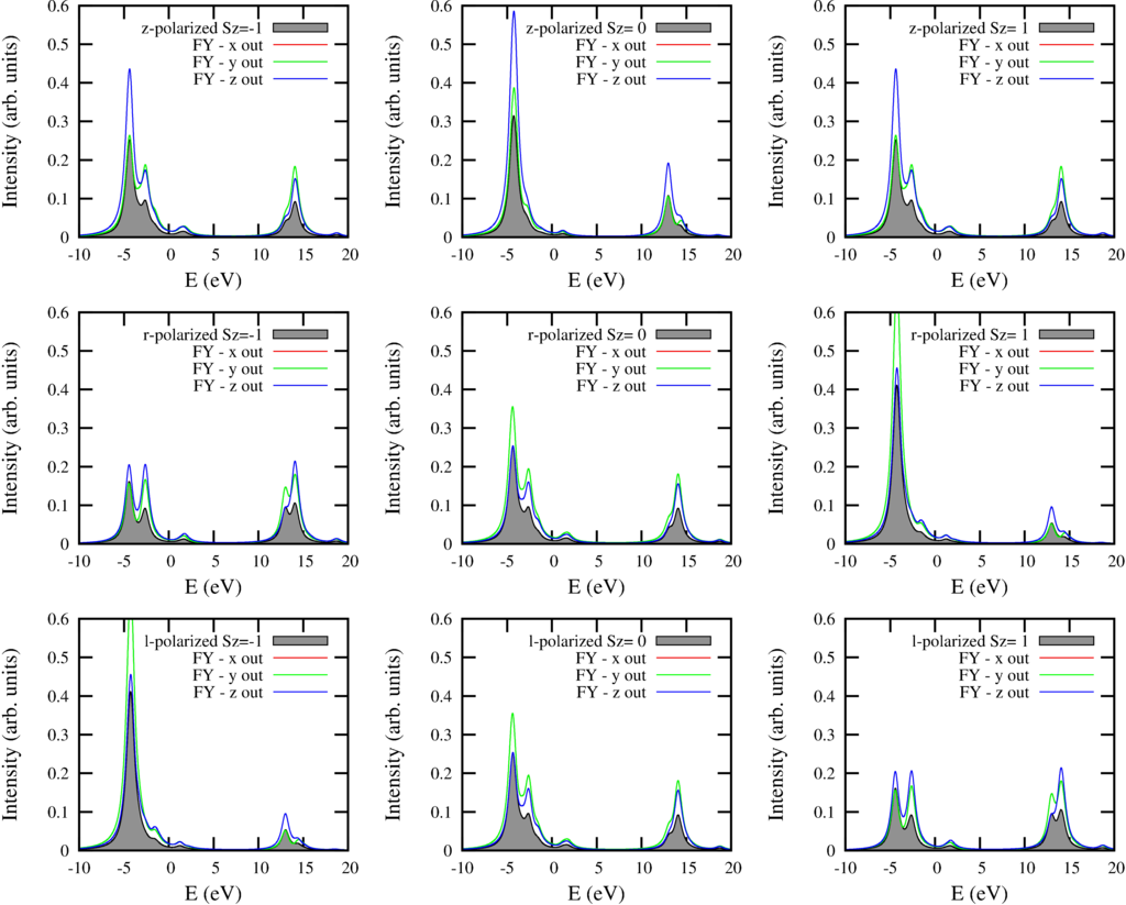 |
| Fluorescence yield spectra for different geometries of both incoming and outgoing polarization compared to x-ray absorbtion |
|---|
The script shows some information on the ground-state, here the text output.
- FY_L23M45.out
  #    <E>      <S^2>    <L^2>    <J^2>    <S_x^3d> <L_x^3d> <S_y^3d> <L_y^3d> <S_z^3d> <L_z^3d> <l.s>    <F[2]>   <F[4]>   <Neg^3d> <Nt2g^3d><Neg^Ld> <Nt2g^Ld><N^3d>
  1   -3.395    1.999   12.000   15.147    0.000    0.000    0.000    0.000   -0.905   -0.280   -0.319   -1.043   -0.925    2.189    5.989    3.823    6.000    8.178
  2   -3.395    1.999   12.000   15.147    0.000    0.000    0.000    0.000   -0.000   -0.000   -0.319   -1.043   -0.925    2.189    5.989    3.823    6.000    8.178
  3   -3.395    1.999   12.000   15.147    0.000    0.000    0.000    0.000    0.905    0.280   -0.319   -1.043   -0.925    2.189    5.989    3.823    6.000    8.178
Start of LanczosTriDiagonalizeKrylovMC
Start of LanczosTriDiagonalizeKrylovMC
Start of LanczosTriDiagonalizeKrylovMC
Start of LanczosTriDiagonalizeKrylovMC
Start of LanczosTriDiagonalizeKrylovMC
Start of LanczosTriDiagonalizeKrylovMC
Start of LanczosTriDiagonalizeKrylovMC
Start of LanczosTriDiagonalizeKrylovMC
Start of LanczosTriDiagonalizeKrylovMC