Table of Contents
Interpolating function
Modified in 0.9.1
An interpolating function is a function $f(x)$ of one real variable made from a table of data points $(x_i, y_i)$, $i = 1 \dots N$. It passes through every data point, $f(x_i) = y_i$, and between the points it is a smooth curve, a polynomial of low degree on each interval. Once made, an interpolating function can be evaluated at any $x$, differentiated, integrated, and combined with other interpolating functions by arithmetic. Outside the interval $[x_1, x_N]$ it is 0, its derivatives as well.
How the curve between the points is chosen, and how smooth it is, depends on the type of the interpolation. Quanty has three types for data, each made by a function of the InterpolatingFunction library, and a fourth type for the radial functions of a relativistic atom, which is made by CalculateAtomicBasisFunctions():
| Type | Made by | Between the points | Continuous | Exact for |
|---|---|---|---|---|
| “Spline” | InterpolatingFunction.Spline(x, y) | cubic polynomials | $f$, $f'$, $f''$ | straight lines; cubics when the slopes at the two ends are given |
| “HermiteCSpline” | InterpolatingFunction.HermiteCSpline(x, y) | cubic polynomials, no overshoot | $f$, $f'$ | straight lines; cubics when the slopes at all points are given |
| “BSpline” | InterpolatingFunction.BSpline(x, y, n) | polynomials of degree $n$ | $f$ up to $f^{(n-1)}$ | polynomials up to degree $n$ |
| “DKBSpline” | CalculateAtomicBasisFunctions() | one component of a radial Dirac spinor | all derivatives | (not made from data) |
Which type to choose:
-
Smooth data: Spline, or a BSpline of higher degree, which converges faster when the points are refined and has more continuous derivatives.
-
Data that must not overshoot, for example a density, an occupation or anything that has to stay positive or monotone: HermiteCSpline. It makes no minima or maxima that the data does not have.
-
Data with known derivatives: HermiteCSpline with the slopes at all points.
-
Straight lines between the points: a BSpline of degree 1.
Example
Modified in 0.9.1
A step, sampled at $x = 0, 1, \dots, 10$, interpolated by a Spline (black), a HermiteCSpline (red) and a BSpline of degree 5 (blue). The cubic spline and the B-spline overshoot near the step and ripple around the flat parts; the higher the degree, the larger the ripples. The Hermite spline stays between 0 and 1. For smooth data the order is reversed: there the B-spline of high degree is the most accurate, see InterpolatingFunction.BSpline().
Input
- Example.Quanty
-- a step sampled at x = 0, 1, ..., 10, interpolated in three ways
x, y = {}, {}
for i = 0, 10 do x[i+1] = i; y[i+1] = (i < 5) and 0 or 1 end
S = InterpolatingFunction.Spline(x, y)
H = InterpolatingFunction.HermiteCSpline(x, y)
B = InterpolatingFunction.BSpline(x, y, 5)

-- the smallest and the largest value between the data points
for _, f in ipairs({S, H, B}) do
  local min, max = 0, 1
  for i = 0, 1000 do
    local v = f(i/100)
    min, max = math.min(min, v), math.max(max, v)
  end
  print(string.format("%-14s degree %d   min %8.4f   max %8.4f", f.type, f.degree, min, max))
end

-- the three curves, and the data as dots
function Curve(f)
  local c = {}
  for i = 0, 400 do c[i+1] = {i/40, f(i/40)} end
  return c
end
Dots = {}
for i = 1, #x do Dots[i] = {x[i], y[i]} end
pl = Graphics.Plot({Curve(S), Curve(H), Curve(B), Dots},
       {{"plotIm", false},
        {"LineStyle", {{}, {}, {}, {{"LineWidth", 0}, {"PointSize", 0.006}, {"PointColor", 0x000000}}}},
        {"Frame", {{"Xmin", 0}, {"Xmax", 10}, {"Ymin", -0.3}, {"Ymax", 1.3}, {"FirstYTick", 0}, {"dYTick", 0.5},
                   {"YFormat", "%.1f"}, {"XLabel", "x"}, {"YLabel", "f(x)"}, {"XLMargin", 0.1}, {"YAxis", -10}}}})
file = io.open("interpolation_types.svg", "w")
file:write(Graphics.ToSVG(pl, {{"RelativeSize", true}}))
file:close()
- Example.out
Spline         degree 3   min  -0.1078   max   1.1078
HermiteCSpline degree 3   min   0.0000   max   1.0000
BSpline        degree 5   min  -0.1343   max   1.1260
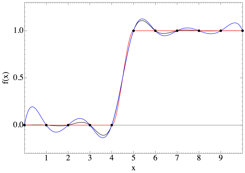
Spline
InterpolatingFunction.Spline(x, y) makes a cubic spline: a cubic polynomial on every interval $[x_i, x_{i+1}]$, joined such that the function, its first and its second derivative are continuous. The natural spline is, of all functions through the points with a continuous second derivative, the one with the least curvature (the smallest integral of $f''^2$), which is why it is the most common interpolation. The two conditions that are still free are set at the ends: $f'' = 0$ (a natural spline), or the slopes $f'(x_1)$ and $f'(x_N)$ given as two extra arguments. The error between the points decreases as $h^4$ with the distance $h$ between the points, when the end conditions are correct. A change of one data point changes the spline everywhere, a little, and near a jump in the data the spline overshoots.
HermiteCSpline
InterpolatingFunction.HermiteCSpline(x, y) makes a cubic Hermite spline: on every interval the cubic polynomial with the values and the slopes at its two ends. The function and its first derivative are continuous, the second derivative jumps at the data points. Without slopes, the slopes are estimated from the neighbouring points and limited (Fritsch–Carlson) such that the interpolation is monotone wherever the data is: there is no overshoot, and a flat part of the data stays flat. With the slopes given at every point, InterpolatingFunction.HermiteCSpline(x, y, m), the slopes are used as they are. The curve between two points only depends on the points nearby, so a change of one data point changes the function only locally.
BSpline
InterpolatingFunction.BSpline(x, y, n) makes a B-spline of degree $n$: a sum of $N$ B-splines $B_j(x)$ of degree $n$, $f(x) = \sum_j c_j B_j(x)$, with the coefficients $c_j$ such that $f$ passes through the $N$ data points. On every interval between two knots $f$ is a polynomial of degree $n$, and $f$ and its derivatives up to order $n-1$ are continuous. The knots are not the data points: the knots inside the interval are averages of $n$ neighbouring data points, and there are $N - n + 1$ different knots. Degree 1 gives straight lines between the points, degree 3 a cubic interpolation that is smooth like a cubic spline, and a higher degree converges faster for smooth data. B-splines are the basis functions of the atomic radial functions of CalculateAtomicBasisFunctions().
DKBSpline
New in 0.9.1
An interpolating function of type “DKBSpline” is not made from data. It is one of the two components of a radial Dirac spinor, as returned by CalculateAtomicBasisFunctions(): the large component $G = P(r) = r g(r)$ or the small component $F = Q(r) = r f(r)$ of an orbital with quantum number $\kappa$. The two belong together. They are expanded in a dual kinetic balance (DKB) B-spline basis (V. M. Shabaev et al., Phys. Rev. Lett. 93, 130405 (2004)), with the two sets of coefficients $a_j$ and $b_j$ of the orbital, $$ \begin{eqnarray} P(r) &=& \sum_j a_j B_j(r) + \frac{1}{2c} \sum_j b_j \left( \frac{d}{dr} - \frac{\kappa}{r} \right) B_j(r), \nonumber \\ Q(r) &=& \sum_j b_j B_j(r) + \frac{1}{2c} \sum_j a_j \left( \frac{d}{dr} + \frac{\kappa}{r} \right) B_j(r), \nonumber \end{eqnarray} $$ with $c$ the speed of light. For an electron the $b_j$ are small and $Q \approx (P' + \kappa P / r)/(2c)$, the kinetic balance of the Dirac equation; the second term of $P$ is the same relation the other way round. Built into the basis, this relation removes the spurious solutions that the radial Dirac equation has in a basis where $P$ and $Q$ are expanded independently.
A DKBSpline therefore has properties of its own:
-
$G$ and $F$ of one orbital share the coefficients; each function knows its $\kappa$, whether it is the large or the small component, and the speed of light it was made with. NewOperator(“Dirac”, …) and NewOperator(“AU”, …) recognise the functions and calculate their matrix elements exactly, and give an error if PhysicalConstants.cAU.value has been changed since.
-
Because of the $1/r$ terms the function is not a polynomial between the knots. f.degree is the degree of the B-splines. Derivatives of every order are calculated exactly from the B-splines.
-
f.x are the radial points of the quadrature of the atom, f.knots the knots of the B-splines, from 0 to the end of the radial grid.
-
In arithmetic (G + F, G * F, …) and comparison a DKBSpline acts as the BSpline of its degree through its values on f.x, and the result is a BSpline: the sum or product of two components is no longer a component of a spinor. The points are dense, so integrals of products, for example the overlap $\int (G_a G_b + F_a F_b) \, \mathrm{d}r$, are exact to rounding.
- Example.Quanty
-- the 2p orbitals of Ne: the large components G and the small components F
G, F, Atom = CalculateAtomicBasisFunctions(10)
c, r = PhysicalConstants.cAU.value, 1
for i, o in ipairs(Atom.Orbitals) do
  if o.l == 1 then
    -- F is close to (G' + kappa G/r)/(2c), the kinetic balance
    print(string.format("%-6s kappa %2d   G(1) = %8.6f   F(1) = %10.7f   (G'(1) + kappa G(1))/(2c) = %10.7f",
                        o.Label, o.kappa, G[i](r), F[i](r), (G[i](r, 1) + o.kappa*G[i](r)/r)/(2*c)))
  end
end
print(string.format("type %s, degree %d, %d knots from %g to %g, %d points x",
                    G[1].type, G[1].degree, #G[1].knots, G[1].knots[1], G[1].knots[#G[1].knots], #G[1].x))
-- the overlaps of 1s1/2 and 2s1/2: the products are BSplines on the points x
print(string.format("<1s|1s> - 1 = %.1e, <1s|2s> = %.1e, type of G * G: %s", InterpolatingFunction.Integrate(G[1]*G[1] + F[1]*F[1]) - 1,
                    InterpolatingFunction.Integrate(G[1]*G[2] + F[1]*F[2]), (G[1]*G[2]).type))
- Example.out
2p1/2  kappa  1   G(1) = 0.831088   F(1) =  0.0009597   (G'(1) + kappa G(1))/(2c) =  0.0009596
2p3/2  kappa -2   G(1) = 0.831407   F(1) = -0.0081275   (G'(1) + kappa G(1))/(2c) = -0.0081277
type DKBSpline, degree 8, 121 knots from 0 to 40, 1560 points x
<1s|1s> - 1 = -2.1e-15, <1s|2s> = -1.8e-16, type of G * G: BSpline
Evaluation
Modified in 0.9.1
An interpolating function f is evaluated as a function:
-
f(t) : the value at $t$.
-
f(t, k) : the $k$-th derivative at $t$. For a cubic spline the derivatives above the third are 0, for a BSpline those above its degree (with a warning).
-
f({t1, t2, …}), f({t1, t2, …}, k) : a table of values. This is faster when the points are in increasing order.
Outside $[x_1, x_N]$ (for a DKBSpline outside its knots) the value and all derivatives are 0.
Properties
Modified in 0.9.1
-
f.x, f.y : the points the function is given on and its values there. For Spline, HermiteCSpline and BSpline these are the data points; a BSpline made from coefficients gives its knots. The radial functions and the potentials of CalculateAtomicBasisFunctions(), of type DKBSpline or BSpline, give the radial points of the quadrature of the atom.
-
f.knots : the points where the polynomial pieces join. For the cubic splines these are the data points.
-
f.degree : the polynomial degree of the pieces, 3 for the cubic splines.
-
f.coefficients : (BSpline only) the B-spline coefficients, one per data point.
-
f.type : the type, “Spline”, “HermiteCSpline”, “BSpline” or “DKBSpline”. For the first three this is the name of the function that made it, so InterpolatingFunction[f.type] makes a function of the same kind.
- Example.Quanty
x = {0, 0.5, 1, 1.5, 2, 2.5, 3}
y = {}
for i = 1, #x do y[i] = math.exp(-x[i]) end
f = InterpolatingFunction.Spline(x, y)
g = InterpolatingFunction.BSpline(x, y, 3)

function List(t)
  local s = {}
  for i = 1, #t do s[i] = string.format("%.4f", t[i]) end
  return "{" .. table.concat(s, ", ") .. "}"
end
print("Spline   x      = " .. List(f.x))
print("Spline   knots  = " .. List(f.knots) .. ", degree " .. f.degree)
print("BSpline  x      = " .. List(g.x))
print("BSpline  y      = " .. List(g.y))
print("BSpline  knots  = " .. List(g.knots) .. ", degree " .. g.degree)
print("BSpline  coefficients = " .. List(g.coefficients))
print("type: " .. f.type .. " and " .. g.type)
- Example.out
Spline   x      = {0.0000, 0.5000, 1.0000, 1.5000, 2.0000, 2.5000, 3.0000}
Spline   knots  = {0.0000, 0.5000, 1.0000, 1.5000, 2.0000, 2.5000, 3.0000}, degree 3
BSpline  x      = {0.0000, 0.5000, 1.0000, 1.5000, 2.0000, 2.5000, 3.0000}
BSpline  y      = {1.0000, 0.6065, 0.3679, 0.2231, 0.1353, 0.0821, 0.0498}
BSpline  knots  = {0.0000, 1.0000, 1.5000, 2.0000, 3.0000}, degree 3
BSpline  coefficients = {1.0000, 0.6713, 0.3996, 0.2139, 0.1018, 0.0670, 0.0498}
type: Spline and BSpline
Arithmetic
Modified in 0.9.1
For two interpolating functions f and g, -f, f + g, f - g, f * g, f / g, f ^ n (with n a number) and the composition f .. g, $f(g(x))$, are again interpolating functions, of the type of f; a DKBSpline acts as the BSpline through its values on its points f.x, so its results are BSplines. Both operands must be interpolating functions; a number is not converted. The result is made on the data points of f and g together (f ^ n and f .. g on those of f), through the exact values $f(x_i) + g(x_i)$, … at these points, and is interpolated between them by the type of f. It is therefore exact at the points, and in general a new approximation between them. Exact everywhere are:
-
f + g and f - g of two Splines: the sum of two cubic splines is a cubic spline on the points of both.
-
-f, and f + g and f - g of two BSplines of the same degree and knots, which act on the coefficients.
For a HermiteCSpline even a sum is a new interpolation, with new slopes. f == g is true when f and g are of the same type and have the same points and values (BSpline: the same degree, knots and coefficients) to a relative precision of $10^{-14}$.
- Example.Quanty
-- two functions on different points
x1, x2 = {0, 0.4, 1.1, 1.6, 2.3, 3}, {0, 0.7, 1.5, 2.2, 3}
function Table(f, x) local y = {} for i = 1, #x do y[i] = f(x[i]) end return y end
for _, name in ipairs({"Spline", "HermiteCSpline"}) do
  local f = InterpolatingFunction[name](x1, Table(math.exp, x1))
  local g = InterpolatingFunction[name](x2, Table(math.sin, x2))
  local s, p = f + g, f * g
  local es, ep = 0, 0
  for i = 0, 300 do
    local t = i/100
    es = math.max(es, math.abs(s(t) - (f(t) + g(t))))
    ep = math.max(ep, math.abs(p(t) - f(t)*g(t)))
  end
  print(string.format("%-14s f+g: %d points, max |(f+g)(t) - f(t) - g(t)| = %.1e;  f*g: max |(f*g)(t) - f(t) g(t)| = %.1e", name, #s.x, es, ep))
end
- Example.out
Spline         f+g: 9 points, max |(f+g)(t) - f(t) - g(t)| = 3.6e-15;  f*g: max |(f*g)(t) - f(t) g(t)| = 7.8e-01
HermiteCSpline f+g: 9 points, max |(f+g)(t) - f(t) - g(t)| = 1.3e-01;  f*g: max |(f*g)(t) - f(t) g(t)| = 1.5e+00
Integration
InterpolatingFunction.Integrate(f) integrates f over its whole interval, InterpolatingFunction.Integrate(f, a, b) from $a$ to $b$. For Spline, HermiteCSpline and BSpline the integral is exact for the interpolating function.
