Density matrix plot
An intuitive way to look at eigenstates is to plot the charge density. For multi-electron wave-functions one can not plot the wave-function (it depends on $3\times n$ coordinates) but the charge density is a well defined simple quantity. We here use the rendering options of \textit{Mathematica} in combination with the package for \textit{Mathematica} (Quanty.nb) to plot the density matrix of the lowest three eigenstates in NiO.
The input script is:
- density_matrix_plots_Mathematica.Quanty
-- It is often nice to make plots of the resulting "wave-functions" Now one can not
-- simply plot a multi-electron wavefunction \psi(r_1,r_2,r_3, ..., r_n) as it depends
-- on 3n coordinates.
-- One can plot the resulting charge density.

-- This example calculates the density matrix of a state and then calls Mathematica to
-- make a density plot of this matrix.

-- the script for mathematica is included in the input file
-- the input string needs calculated data which will be substituted before calling mathematica

Verbosity(0)

-- You need to change the absolute path in the script below
mathematicaInput = [[
Needs["Quanty`PlotTools`"];
rho=%s;
pl = Table[ Rasterize[ DensityMatrixPlot[IdentityMatrix[10] - rho[ [i] ], PlotRange -> {{-0.4, 0.4}, {-0.4, 0.4}, {-0.4, 0.4}}] ], {i, 1, Length[rho]}];
For[i = 1, i <= Length[pl], i++,
    Export["/Users/haverkort/Documents/Quanty/Example_and_Testing/History/current/Tutorials/20_NiO_Crystal_Field/Rho" <> ToString[i] <> ".png", pl[ [i] ] ];
   ];
Quit[];
]]

NF=10
NB=0
dIndexDn={0,2,4,6,8}
dIndexUp={1,3,5,7,9}

OppSx   =NewOperator("Sx"   ,NF, dIndexUp, dIndexDn)
OppSy   =NewOperator("Sy"   ,NF, dIndexUp, dIndexDn)
OppSz   =NewOperator("Sz"   ,NF, dIndexUp, dIndexDn)
OppSsqr =NewOperator("Ssqr" ,NF, dIndexUp, dIndexDn)
OppSplus=NewOperator("Splus",NF, dIndexUp, dIndexDn)
OppSmin =NewOperator("Smin" ,NF, dIndexUp, dIndexDn)

OppLx   =NewOperator("Lx"   ,NF, dIndexUp, dIndexDn)
OppLy   =NewOperator("Ly"   ,NF, dIndexUp, dIndexDn)
OppLz   =NewOperator("Lz"   ,NF, dIndexUp, dIndexDn)
OppLsqr =NewOperator("Lsqr" ,NF, dIndexUp, dIndexDn)
OppLplus=NewOperator("Lplus",NF, dIndexUp, dIndexDn)
OppLmin =NewOperator("Lmin" ,NF, dIndexUp, dIndexDn)

OppJx   =NewOperator("Jx"   ,NF, dIndexUp, dIndexDn)
OppJy   =NewOperator("Jy"   ,NF, dIndexUp, dIndexDn)
OppJz   =NewOperator("Jz"   ,NF, dIndexUp, dIndexDn)
OppJsqr =NewOperator("Jsqr" ,NF, dIndexUp, dIndexDn)
OppJplus=NewOperator("Jplus",NF, dIndexUp, dIndexDn)
OppJmin =NewOperator("Jmin" ,NF, dIndexUp, dIndexDn)

Oppldots=NewOperator("ldots",NF, dIndexUp, dIndexDn)

-- define the coulomb operator
-- we here define the part depending on F0 seperately from the part depending on F2
-- when summing we can put in the numerical values of the slater integrals
OppF0 =NewOperator("U", NF, dIndexUp, dIndexDn, {1,0,0})
OppF2 =NewOperator("U", NF, dIndexUp, dIndexDn, {0,1,0})
OppF4 =NewOperator("U", NF, dIndexUp, dIndexDn, {0,0,1})

-- Akm = {{k1,m1,Akm1},{k2,m2,Akm2}, ... }
Akm = PotentialExpandedOnClm("Oh", 2, {0.6,-0.4})
OpptenDq = NewOperator("CF", NF, dIndexUp, dIndexDn, Akm)

Akm = PotentialExpandedOnClm("Oh", 2, {1,0})
OppNeg = NewOperator("CF", NF, dIndexUp, dIndexDn, Akm)
Akm = PotentialExpandedOnClm("Oh", 2, {0,1})
OppNt2g = NewOperator("CF", NF, dIndexUp, dIndexDn, Akm)

Hamiltonian =  10.0 * OppF2 + 6.25 * OppF4 + 2.0 * OpptenDq + 0.06 * Oppldots + 0.000001 * (2*OppSz + OppLz)

-- we now can create the lowest Npsi eigenstates:
Npsi=3
-- in order to make sure we have a filling of 2 electrons we need to define some restrictions
StartRestrictions = {NF, NB, {"1111111111",8,8}}

psiList = Eigensystem(Hamiltonian, StartRestrictions, Npsi)
oppList={Hamiltonian, OppSsqr, OppLsqr, OppJsqr, OppSz, OppLz, Oppldots, OppF2, OppF4, OppNeg, OppNt2g}

print(" <E>    <S^2>  <L^2>  <J^2>  <S_z>  <L_z>  <l.s>  <F[2]> <F[4]> <Neg>  <Nt2g>");
for key,psi in pairs(psiList) do
  expvalue = psi * oppList * psi
  for k,v in pairs(expvalue) do
    io.write(string.format("%6.3f ",v))
  end;
  io.write("\n")
end
io:flush()

function tableToMathematica(t)
  local ret = "{ "
  for k,v in pairs(t) do
    if k~=1 then
      ret = ret.." , "
    end
    if (type(v) == "table") then
      ret = ret..tableToMathematica(v)
    else
      ret = ret..string.format("%18.15f + (%18.15f) I ",Complex.Re(v),Complex.Im(v))
    end
  end
  ret = ret.." }"
  return ret
end

rhoList = DensityMatrix(psiList, {0,1,2,3,4,5,6,7,8,9})
rhoListMathematicaForm = tableToMathematica(rhoList)

file = io.open("densitymatrix.nb", "w")
file:write( mathematicaInput:format( rhoListMathematicaForm ) )
file:close()

os.execute("/Applications/Mathematica08.app/Contents/MacOS/MathKernel -run '<<densitymatrix.nb'")
os.execute("convert Rho1.png -transparent white temp.png ; convert temp.png Rho1.eps ; rm temp.png")
os.execute("convert Rho2.png -transparent white temp.png ; convert temp.png Rho2.eps ; rm temp.png")
os.execute("convert Rho3.png -transparent white temp.png ; convert temp.png Rho3.eps ; rm temp.png")
The produced figures are:
| $S_z=-1$ | $S_z=0$ | $S_z=1$ |
|---|---|---|
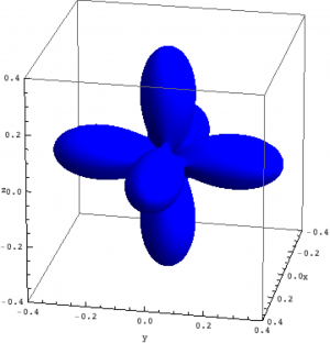 | 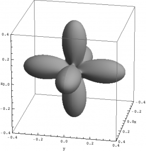 | 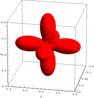 |
| Density matrix of the ground, first and second excited state of Ni in NiO. | ||
The plots can be seen in the figure above. We show the hole density (identity matrix minus the density matrix) which has lobes towards the O atoms. Ni in NiO has a hole in the $x^2-y^2$ and in the $z^2$ orbital. The color represent the spin down, $S_z=0$ and spin up state of the lowest triplet.
The output to the screen is:
- density_matrix_plots_Mathematica.out
 <E>    <S^2>  <L^2>  <J^2>  <S_z>  <L_z>  <l.s>  <F[2]> <F[4]> <Neg>  <Nt2g>
-18.093  2.000 12.000 14.471 -0.999 -0.119 -0.147 -1.020 -0.878  2.002  5.998
-18.093  2.000 12.000 14.471 -0.000 -0.000 -0.147 -1.020 -0.878  2.002  5.998
-18.093  2.000 12.000 14.471  0.999  0.119 -0.147 -1.020 -0.878  2.002  5.998
Mathematica 8.0 for Mac OS X x86 (64-bit)
Copyright 1988-2011 Wolfram Research, Inc.
Loaded the Quanty : Plot Tools Package - version 2016.4.13
Written by Maurits W. Haverkort