This is an old revision of the document!
RIXS $L_{2,3}M_{1}$
Instead of looking at low energy excitations one can use RIXS to look at core-core excitations. A powerful technique comparable to other core level spectroscopies like x-ray absorption and core-level photoemission at once.
Here a script to calculate the Ni $2p$ to $3d$ excitation ($L_{2,3}$) and Ni $3s$ to $2p$ decay ($M_{1}$).
- RIXS_L23M1.Quanty
-- This example calculates core - core RIXS spectra. These type of spectra are
-- highly informative and contain similar information as core level absorption and
-- core level photoemission combined. With generally enhances sensitivity.

-- we focus here on 2p to 3d excitations (L23) and 3s to 2p decay (final hole in the 3s
-- state, the M1 edge)

-- we minimize the output by setting the verbosity to 0
Verbosity(0)

-- We need the 2p, 3s and 3d shell in the basis
NF=18
NB=0
IndexDn_2p={0,2,4}
IndexUp_2p={1,3,5}
IndexDn_3s={6}
IndexUp_3s={7}
IndexDn_3d={8,10,12,14,16}
IndexUp_3d={9,11,13,15,17}

-- just like in the previous example we define several operators acting on the Ni -3d shell

OppSx   =NewOperator("Sx"   ,NF, IndexUp_3d, IndexDn_3d)
OppSy   =NewOperator("Sy"   ,NF, IndexUp_3d, IndexDn_3d)
OppSz   =NewOperator("Sz"   ,NF, IndexUp_3d, IndexDn_3d)
OppSsqr =NewOperator("Ssqr" ,NF, IndexUp_3d, IndexDn_3d)
OppSplus=NewOperator("Splus",NF, IndexUp_3d, IndexDn_3d)
OppSmin =NewOperator("Smin" ,NF, IndexUp_3d, IndexDn_3d)

OppLx   =NewOperator("Lx"   ,NF, IndexUp_3d, IndexDn_3d)
OppLy   =NewOperator("Ly"   ,NF, IndexUp_3d, IndexDn_3d)
OppLz   =NewOperator("Lz"   ,NF, IndexUp_3d, IndexDn_3d)
OppLsqr =NewOperator("Lsqr" ,NF, IndexUp_3d, IndexDn_3d)
OppLplus=NewOperator("Lplus",NF, IndexUp_3d, IndexDn_3d)
OppLmin =NewOperator("Lmin" ,NF, IndexUp_3d, IndexDn_3d)

OppJx   =NewOperator("Jx"   ,NF, IndexUp_3d, IndexDn_3d)
OppJy   =NewOperator("Jy"   ,NF, IndexUp_3d, IndexDn_3d)
OppJz   =NewOperator("Jz"   ,NF, IndexUp_3d, IndexDn_3d)
OppJsqr =NewOperator("Jsqr" ,NF, IndexUp_3d, IndexDn_3d)
OppJplus=NewOperator("Jplus",NF, IndexUp_3d, IndexDn_3d)
OppJmin =NewOperator("Jmin" ,NF, IndexUp_3d, IndexDn_3d)

Oppldots=NewOperator("ldots",NF, IndexUp_3d, IndexDn_3d)

-- as in the previous example we define the Coulomb interaction
OppF0 =NewOperator("U", NF, IndexUp_3d, IndexDn_3d, {1,0,0})
OppF2 =NewOperator("U", NF, IndexUp_3d, IndexDn_3d, {0,1,0})
OppF4 =NewOperator("U", NF, IndexUp_3d, IndexDn_3d, {0,0,1})

-- as in the previous example we define the crystal-field operator
Akm = PotentialExpandedOnClm("Oh", 2, {0.6,-0.4})
OpptenDq = NewOperator("CF", NF, IndexUp_3d, IndexDn_3d, Akm)

-- and as in the previous example we define operators that count the number of eg and t2g
-- electrons
Akm = PotentialExpandedOnClm("Oh", 2, {1,0})
OppNeg = NewOperator("CF", NF, IndexUp_3d, IndexDn_3d, Akm)
Akm = PotentialExpandedOnClm("Oh", 2, {0,1})
OppNt2g = NewOperator("CF", NF, IndexUp_3d, IndexDn_3d, Akm)

-- In order te describe the resonance we need the interaction on the 2p shell (spin-orbit)
Oppcldots= NewOperator("ldots", NF, IndexUp_2p, IndexDn_2p)

-- and the Coulomb interaction between the 2p and 3d shell
OppUpdF0 = NewOperator("U", NF, IndexUp_2p, IndexDn_2p, IndexUp_3d, IndexDn_3d, {1,0}, {0,0})
OppUpdF2 = NewOperator("U", NF, IndexUp_2p, IndexDn_2p, IndexUp_3d, IndexDn_3d, {0,1}, {0,0})
OppUpdG1 = NewOperator("U", NF, IndexUp_2p, IndexDn_2p, IndexUp_3d, IndexDn_3d, {0,0}, {1,0})
OppUpdG3 = NewOperator("U", NF, IndexUp_2p, IndexDn_2p, IndexUp_3d, IndexDn_3d, {0,0}, {0,1})

-- and the Coulomb interaction between the 3s and 3d shell (new here, needed for the final state)
-- note that in the fluoressence yield example we did not need this interaction as the
-- spectra were integrated over all outgoing photon energies
OppUsdF0 = NewOperator("U", NF, IndexUp_3s, IndexDn_3s, IndexUp_3d, IndexDn_3d, {1}, {0})
OppUsdG2 = NewOperator("U", NF, IndexUp_3s, IndexDn_3s, IndexUp_3d, IndexDn_3d, {0}, {1})

-- next we define the dipole operator. The dipole operator is given as epsilon.r
-- with epsilon the polarization vector of the light and r the unit position vector
-- We can expand the position vector on (renormalized) spherical harmonics and use
-- the crystal-field operator to create the dipole operator.

-- we both define the dipole operator between the 2p and 3d shell as well as the dipole
-- operator between the 3s and 2p shell

-- x polarized light is defined as x = Cos[phi]Sin[theta] = sqrt(1/2) ( C_1^{(-1)} - C_1^{(1)})
Akm = {{1,-1,sqrt(1/2)},{1, 1,-sqrt(1/2)}}
TXASx  = NewOperator("CF", NF, IndexUp_3d, IndexDn_3d, IndexUp_2p, IndexDn_2p, Akm)
T3s2px = NewOperator("CF", NF, IndexUp_2p, IndexDn_2p, IndexUp_3s, IndexDn_3s, Akm)
-- y polarized light is defined as y = Sin[phi]Sin[theta] = sqrt(1/2) I ( C_1^{(-1)} + C_1^{(1)})
Akm = {{1,-1,sqrt(1/2)*I},{1, 1,sqrt(1/2)*I}}
TXASy  = NewOperator("CF", NF, IndexUp_3d, IndexDn_3d, IndexUp_2p, IndexDn_2p, Akm)
T3s2py = NewOperator("CF", NF, IndexUp_2p, IndexDn_2p, IndexUp_3s, IndexDn_3s, Akm)
-- z polarized light is defined as z = Cos[theta] = C_1^{(0)}
Akm = {{1,0,1}}
TXASz  = NewOperator("CF", NF, IndexUp_3d, IndexDn_3d, IndexUp_2p, IndexDn_2p, Akm)
T3s2pz = NewOperator("CF", NF, IndexUp_2p, IndexDn_2p, IndexUp_3s, IndexDn_3s, Akm)

-- besides linear polarized light one can define circular polarized light as the sum of
-- x and y polarizations with complex prefactors
TXASr = sqrt(1/2)*(TXASx - I * TXASy)
TXASl =-sqrt(1/2)*(TXASx + I * TXASy)

-- we can remove zero's from the dipole operator by chopping it.
TXASr.Chop()
TXASl.Chop()

-- once all operators are defined we can set some parameter values.

-- the value of U drops out of a crystal-field calculation as the total number of electrons
-- is always the same
U       =  0.000
-- F2 and F4 are often referred to in the literature as J_{Hund}. They represent the energy
-- differences between different multiplets. Numerical values can be found in the back of
-- my PhD. thesis for example. http://arxiv.org/abs/cond-mat/0505214
F2dd    = 11.142
F4dd    =  6.874
-- F0 is not the same as U, although they are related. Unimportant in crystal-field theory
-- the difference between U and F0 is so important that I do include it here. (U=0 so F0 is not)
F0dd    = U+(F2dd+F4dd)*2/63
-- in crystal field theory U drops out of the equation, also true for the interaction between the
-- Ni 2p and Ni 3d electrons
Upd     =  0.000
-- The Slater integrals between the 2p and 3d shell, again the numerical values can be found
-- in the back of my PhD. thesis. (http://arxiv.org/abs/cond-mat/0505214)
F2pd    =  6.667
G1pd    =  4.922
G3pd    =  2.796
-- F0 is not the same as U, although they are related. Unimportant in crystal-field theory
-- the difference between U and F0 is so important that I do include it here. (U=0 so F0 is not)
F0pd    =  Upd + G1pd*1/15 + G3pd*3/70
-- We now also need the interaction between the 3s and 3d orbital
Usd     =  0.000
G2sd    = 12.560
-- and again F0 is not equal to U, so include the difference
F0sd    =  Usd + G2sd/10
-- tenDq in NiO is 1.1 eV as can be seen in optics or using IXS to measure d-d excitations
tenDq   =  1.100
-- the Ni 3d spin-orbit is small but finite
zeta_3d =  0.081
-- the Ni 2p spin-orbit is very large and should not be scaled as theory is quite accurate here
zeta_2p = 11.498
-- we can add a small magnetic field, just to get nice expectation values. (units in eV... )
Bz      = 0.000001

-- the total Hamiltonian is the sum of the different operators multiplied with their prefactor
Hamiltonian = F0dd*OppF0 + F2dd*OppF2 + F4dd*OppF4 + tenDq*OpptenDq + zeta_3d*Oppldots + Bz*(2*OppSz+OppLz)

-- We normally do not include core-valence interactions between filed and partially filled
-- shells as it drops out anyhow. For the XAS we thus need to define a "different"
-- (more complete) Hamiltonian.
XASHamiltonian = Hamiltonian + zeta_2p * Oppcldots + F0pd * OppUpdF0 + F2pd * OppUpdF2 + G1pd * OppUpdG1 + G3pd * OppUpdG3

-- we now also need the Hamiltonian for the configuration with a core hole in the 3s state
-- here it is:
Hamiltonian3s = Hamiltonian + F0sd * OppUsdF0 + G2sd * OppUsdG2


-- We saw in the previous example that NiO has a ground-state doublet with occupation
-- t2g^6 eg^2 and S=1 (S^2=S(S+1)=2). The next state is 1.1 eV higher in energy and thus
-- unimportant for the ground-state upto temperatures of 10 000 Kelvin. We thus restrict
-- the calculation to the lowest 3 eigenstates.
Npsi=3
-- We need a filling of 6 electrons in the 2p shell
-- 2 electrons in the 3s shell
-- and 8 electrons in the 3d shell
StartRestrictions = {NF, NB, {"111111 11 0000000000",8,8}, {"000000 00 1111111111",8,8}}

-- And calculate the lowest 3 eigenfunctions
psiList = Eigensystem(Hamiltonian, StartRestrictions, Npsi)

-- In order to get some information on these eigenstates it is good to plot expectation values
-- We first define a list of all the operators we would like to calculate the expectation value of
oppList={Hamiltonian, OppSsqr, OppLsqr, OppJsqr, OppSz, OppLz, Oppldots, OppF2, OppF4, OppNeg, OppNt2g};

-- next we loop over all operators and all states and print the expectation value
print(" <E>    <S^2>  <L^2>  <J^2>  <S_z>  <L_z>  <l.s>  <F[2]> <F[4]> <Neg>  <Nt2g>");
for i = 1,#psiList do
  for j = 1,#oppList do
    expectationvalue = Chop(psiList[i]*oppList[j]*psiList[i])
    io.write(string.format("%8.3f ",Complex.Re(expectationvalue)))
  end
  io.write("\n")
end

-- spectra XAS
XASSpectra = CreateSpectra(XASHamiltonian, TXASx, psiList[1], {{"Emin",-10}, {"Emax",20}, {"NE",3500}, {"Gamma",1.0}})
XASSpectra.Print({{"file","RIXSL23M1_XAS.dat"}})

-- spectra FY
FYSpectra = CreateFluorescenceYield(XASHamiltonian, TXASx, T3s2py, psiList[1], {{"Emin",-10}, {"Emax",20}, {"NE",3500}, {"Gamma",1.0}})
FYSpectra.Print({{"file","RIXSL23M1_FY.dat"}})

-- spectra RIXS
RIXSSpectra = CreateResonantSpectra(XASHamiltonian, Hamiltonian3s, TXASx, T3s2py, psiList[1], {{"Emin1",-10}, {"Emax1",20}, {"NE1",120}, {"Gamma1",1.0}, {"Emin2",-1}, {"Emax2",9}, {"NE2",1000}, {"Gamma2",0.5}})
RIXSSpectra.Print({{"file","RIXSL23M1.dat"}})

print("Finished calculating the spectra now start plotting.\nThis might take more time than the calculation");

-- and make some plots
gnuplotInput = [[
set autoscale
set xtic auto
set ytic auto
set style line  1 lt 1 lw 1 lc rgb "#000000"
set style line  2 lt 1 lw 1 lc rgb "#FF0000"
set style line  3 lt 1 lw 1 lc rgb "#00FF00"
set style line  4 lt 1 lw 1 lc rgb "#0000FF"

set out 'RIXSL23M1_Map.ps'
set terminal postscript portrait enhanced color  "Times" 8 size 7.5,6

unset colorbox

energyshift=857.6
energyshiftM1=110.8

set multiplot
set size 0.5,0.55
set origin 0,0

set ylabel "resonant energy (eV)" font "Times,10"
set xlabel "energy loss (eV)" font "Times,10"

set yrange [852:860]
set xrange [energyshiftM1-0.5:energyshiftM1+7.5]

plot "<(awk '((NR>5)&&(NR<1007)){for(i=3;i<=NF;i=i+2){printf \"%s \", $i}{printf \"%s\", RS}}' RIXSL23M1.dat)" matrix using ($2/100-1.0+energyshiftM1):($1/4+energyshift-10):(-$3) with image notitle

set origin 0.5,0

set yrange [869:877]
set xrange [energyshiftM1-0.5:energyshiftM1+7.5]

plot "<(awk '((NR>5)&&(NR<1007)){for(i=3;i<=NF;i=i+2){printf \"%s \", $i}{printf \"%s\", RS}}' RIXSL23M1.dat)" matrix using ($2/100-1.0+energyshiftM1):($1/4+energyshift-10):(-$3) with image notitle

unset multiplot

set out 'RIXSL23M1_Spec.ps'
set size 1.0, 1.0
set terminal postscript portrait enhanced color  "Times" 8 size 7.5,5

set multiplot
set size 0.25,1.0
set origin 0,0

set ylabel "E (eV)" font "Times,10"
set xlabel "XAS" font "Times,10"
set yrange [energyshift-10:energyshift+20]
set xrange [-0.3:0]
plot "RIXSL23M1_XAS.dat"  using       3:($1+energyshift) notitle with lines ls  1,\
     "RIXSL23M1_FY.dat"   using (-5*$2):($1+energyshift) notitle with lines ls  4

set size 0.8,1.0
set origin 0.2,0.0

set xlabel "Energy loss (eV)" font "Times,10"
unset ylabel
unset ytics
set xrange [energyshiftM1-0.5:energyshiftM1+7.5]

ofset = 0.25
scale=10

plot for [i=0:120] "RIXSL23M1.dat"  using ($1+energyshiftM1):(-column(3+2*i)*scale+ofset*i-10 + energyshift) notitle with lines ls  4

unset multiplot
]]

-- write the gnuplot script to a file
file = io.open("RIXSL23M1.gnuplot", "w")
file:write(gnuplotInput)
file:close()


-- call gnuplot to execute the script
os.execute("gnuplot RIXSL23M1.gnuplot")
-- transform to pdf and eps
os.execute("ps2pdf RIXSL23M1_Map.ps  ; ps2eps RIXSL23M1_Map.ps  ;  mv RIXSL23M1_Map.eps temp.eps  ; eps2eps temp.eps RIXSL23M1_Map.eps  ; rm temp.eps")
os.execute("ps2pdf RIXSL23M1_Spec.ps ; ps2eps RIXSL23M1_Spec.ps ;  mv RIXSL23M1_Spec.eps temp.eps ; eps2eps temp.eps RIXSL23M1_Spec.eps ; rm temp.eps")
Just like in the case of $L_{2,3}M_{4,5}$ edge RIXS we can make plots:
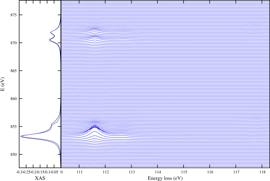
The first shows on the left the XAS spectra in black and the integrated RIXS spectra (FY) in blue. The core-core RIXS is shown on the right.
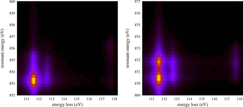
The second plot shows the same RIXS spectra, but now as an intensity map.
The output of the script is:
- RIXS_L23M1.out
 <E>    <S^2>  <L^2>  <J^2>  <S_z>  <L_z>  <l.s>  <F[2]> <F[4]> <Neg>  <Nt2g>
-2.721  1.999 12.000 15.120 -0.994 -0.286 -0.324 -1.020 -0.878  2.011  5.989
-2.721  1.999 12.000 15.120 -0.000 -0.000 -0.324 -1.020 -0.878  2.011  5.989
-2.721  1.999 12.000 15.120  0.994  0.286 -0.324 -1.020 -0.878  2.011  5.989
Start of LanczosTriDiagonalizeKrylovRR
Start of LanczosTriDiagonalizeKrylovRR
Finished calculating the spectra now start plotting.
This might take more time than the calculation