Table of Contents
Plot
pl = Graphics.Plot(Data, Options) plots spectra, lists of data points and response functions and returns a Graphics object, an A4 page in landscape with a frame, axes and the curves. Graphics.ToSVG(pl) and Graphics.ToPS(pl) turn it into the text of an svg or a PostScript file. pl = Graphics.Plot(G, GammaL, GammaG, NE, Options) plots a response function, broadened. Several curves can be drawn in one frame, as a waterfall plot shifted above each other, as a color map, or as a grid of panels.
Input
-
Data : one of
-
a Spectra object, as made by CreateSpectra, CreateResonantSpectra or ResponseFunction.ToSpectra. A Spectra object with several spectra is drawn as several curves.
-
a list of points { {x1, y1}, {x2, y2}, …}. The points are drawn at their own x and joined in the order of the list, so they need not be equally spaced. The y are real or complex numbers; a real y is the real part, so a list of real data is plotted with {“plotIm”,false}.
-
a list of curves, {C1, C2, …}, each a Spectra object, a list of points or a response function. The response functions are broadened by the fields GammaL and GammaG of the list, {C1, C2, …, GammaL = 0.2}, and evaluated at “PlotPoints” energies of the plot range.
G : a response function. It is evaluated at the energies of the plot range, from “Xmin” to “Xmax” of the “Frame”, by default from -1 to 1. A matrix valued (block) response function is drawn as a grid of panels, one for each matrix element.GammaL : (optional) Real, the Lorentzian broadening of G (full width at half maximum). Default value 0GammaG : (optional) Real, the Gaussian broadening of G (full width at half maximum). Default value 0NE : (optional) Integer, the number of energies at which G is evaluated. Default value $1 + 10 (X_{max} - X_{min}) / \Gamma$, with $\Gamma$ = GammaL, or GammaG when GammaL is 0, and “PlotPoints” when both are 0Options : A table of options. Possible options are:-
“Frame” : a table of options for the frame and the axes, see The frame below. “Axis” is the same option.
-
“plotRe” : Boolean, draw the real part. Default value true
-
“plotIm” : Boolean, draw the imaginary part. Default value true
-
“Negate” : Boolean, draw minus the values, for example $-\mathrm{Im}\,G$ for an intensity. Default value false
-
“Scale” : Real, the values are multiplied by “Scale” before they are drawn. Default value 1
-
“LineStyle” : a list of line styles, see Line styles below
-
“LineStyleCycle” : Integer, the curves of a list take the styles 1 to “LineStyleCycle” in turn. Default value: all styles
-
“PlotPoints” : Integer, the number of energies at which the response functions in a list are evaluated. Default value 600
-
“WaterfallShift” : Real, curve $n$ is shifted up by $(n-1)$ “WaterfallShift”. Default value 0
-
“WaterfallOffset” : Real, all curves are shifted up by “WaterfallOffset”. Default value 0
-
“UseResonantEnergy” : Boolean, each spectrum of a Spectra object made by CreateResonantSpectra is shifted up to “WaterfallOffset” plus its resonant energy, the incoming energy of a RIXS spectrum. Can not be combined with “WaterfallShift”. Default value false
-
“SpectraStart”, “SpectraStop”, “SpectraStep” : Integers, plot only the curves SpectraStart, SpectraStart + SpectraStep, … up to SpectraStop, as in a Lua loop for n = Start, Stop, Step. The curves are counted from 1; the elements of a matrix valued response function are counted row by row. Default values 1, the last curve and 1
-
“Nrow”, “Ncolumn” : Integers, draw a Spectra object of Nrow · Ncolumn spectra as a grid of panels. Default values 1 and 1
-
“ScaleOffDiagonal”, “ShiftOffDiagonal” : Reals, the vertical range of the off-diagonal panels of a grid, see Grids of panels below. Default values 1 and 0
-
“ColorMap” : Boolean, draw the curves as a color map instead of lines, see Color maps below. Default value false
-
“NPixelX”, “NPixelY” : Integers, the number of pixels of a color map. Default values 600 and 600
-
“Interpolate” : Boolean, interpolate a color map linearly between the energies and between the curves. Default value true
-
“Color” : 32 bit integer 0xAARRGGBB, the color of the built-in color scale of a color map. Default value 0x000000 (black)
-
“Saturation” : Real, the scale of the built-in color scale. Default value 1
-
“ColorFunction” : a function r, g, b = f(Re, Im) that gives a color map its own color scale
Output
-
pl : a Graphics object, an A4 page in landscape (297 mm by 210 mm).
The frame
The option “Frame” is a table of options:
-
“Xmin”, “Xmax”, “Ymin”, “Ymax” : Reals, the plot range. Without “Xmin” and “Xmax” the range covers the spectra and the lists of points; a response function is evaluated from -1 to 1, also in a list together with spectra, so give “Xmin” and “Xmax” when plotting one. Without “Ymin” and “Ymax” the range is -1 to 1, except for waterfall plots and color maps, where it covers all curves.
-
“XLabel”, “YLabel” : Strings, the labels of the axes. Default value “”
-
“FirstXTick”, “dXTick”, “NMinorXTick” : the first labelled tick (default “Xmin”), the distance between two labelled ticks (default 1) and the number of small ticks between them (default 9). A tick that lies exactly on the edge of the frame gets no number. The same for Y.
-
“XFormat”, “YFormat” : Strings, how the numbers at the ticks are written, as in string.format. Default value “%.0f”
-
“XTicks”, “YTicks” : Booleans, draw the ticks and their numbers. Default value true
-
“XAxis”, “YAxis” : Reals, the height of a horizontal line and the position of a vertical line through the plot. Outside the plot range they are not drawn, so {“YAxis”,-10} leaves the vertical line out. Default value 0
-
“XLMargin”, “XRMargin” : Reals, the room left and right of the frame, as a fraction of the width of the page. Default values 0.08 and 0.01
-
“YLMargin”, “YRMargin” : Reals, the room below and above the frame, as a fraction of the height of the page. Default values 0.113 and 0.014. The labels of the axes are written in the left and the bottom margin.
-
“LineWidth” : Real, the width of the lines of the frame. Default value 0.001
-
“Color” : 32 bit integer 0xAARRGGBB, the color of the frame. Default value 0x000000 (black)
-
“FontSize” : Real, the height of the numbers and the labels. Default value 0.04
-
“Font” : String, the PostScript name of the font. Default value “TimesNewRomanPSMT”
Line styles
The option “LineStyle” is a list of styles, {style1, style2, …}, each a table of options:
-
“LineWidth” : Real, the width of the line, as a fraction of $\sqrt{\mathrm{width} \cdot \mathrm{height}}$ of the page; 0 for no line. Default value 0.002
-
“LineColor” : 32 bit integer 0xAARRGGBB, the color of the line
-
“PointSize” : Real, the radius of a dot at each data point; 0 for no dots. Default value 0
-
“PointColor” : 32 bit integer 0xAARRGGBB, the color of the dots
There are always at least three styles: style 1 is black, style 2 red and style 3 blue. A style given in “LineStyle” changes only the options it names, so {“LineStyle”, {[2] = { {“LineColor”,0x00A000}}}}, or {“LineStyle”, { {}, { {“LineColor”,0x00A000}}}}, makes style 2 green and keeps the width of style 2 and the styles 1 and 3. A style beyond the third that is not given is a copy of the default style 1.
Which style goes to which curve:
-
a single curve with only its real or only its imaginary part takes style 1;
-
a single curve with both parts takes style 2 for the real part and style 3 for the imaginary part;
-
several curves in one frame, with only the real or only the imaginary part: curve $n$ takes style $n$;
-
several curves in one frame with both parts: curve $n$ takes style $2n-1$ for its real part and style $2n$ for its imaginary part;
-
a grid of panels: each panel holds a single curve and takes the styles of a single curve.
When the curves of a list run out of styles they start again from style 1. They cycle through all styles, at least three, or through the first “LineStyleCycle” styles. Two colors that alternate therefore need “LineStyleCycle”: {“LineStyle”, {Orange, Green}} alone gives orange, green, blue (the default style 3), orange, …; with {“LineStyleCycle”,2} it gives orange, green, orange, green, … “LineStyleCycle” can not be larger than the number of styles.
Waterfall plots
With “WaterfallShift” or “UseResonantEnergy” the curves of a list are drawn above each other: curve $n$ at WaterfallOffset + $(n-1)$ WaterfallShift, or at WaterfallOffset plus its resonant energy. The values are multiplied by “Scale” before they are shifted. With “UseResonantEnergy” the vertical axis reads the incoming energy of RIXS spectra, also when the incoming energies are not equally spaced. “UseResonantEnergy” needs a Spectra object and can not be combined with “Nrow” and “Ncolumn”.
Color maps
With {“ColorMap”,true} the curves of a list are drawn as a color map, a bitmap of “NPixelX” by “NPixelY” pixels inside the frame. Each curve lies at the height it would have in a waterfall plot, or, without the waterfall options, at its number $n$. The heights must increase or decrease from curve to curve, and a color map needs at least two curves on a common energy mesh: it can not be made of lists of points, and not combined with “Nrow” and “Ncolumn”. With “Interpolate” the map is interpolated linearly in energy and between neighboring curves; without it each pixel takes the nearest point, the boundary between two curves lies half way between them, and the pixels are drawn as sharp squares.
The value at a pixel is the imaginary part, or the real part with {“plotIm”,false}, after “Negate” and “Scale”. The built-in color scale goes from white to “Color” as “Saturation” times the value goes from 0 to 1. A “ColorFunction” f(Re, Im) gets both parts and returns red, green and blue, each from 0 to 1 (values outside are clipped); it can show the intensity on a scale of its own, a logarithmic scale, or the sign or the phase of a response function.
Grids of panels
A matrix valued response function, and a Spectra object with “Nrow” and “Ncolumn”, is drawn as a grid of panels, one curve each, with the first curve (the element $G_{11}$) in the top left corner, row by row. All panels share the plot range of the “Frame”. The off-diagonal panels can show a different vertical range: from $(Y_{min} - s)\, c$ to $(Y_{max} - s)\, c$, with $s$ = “ShiftOffDiagonal” and $c$ = “ScaleOffDiagonal”, so that $c < 1$ magnifies the off-diagonal elements by $1/c$. The numbers on the vertical axis are those of the diagonal panels. To draw some of the elements in one frame instead, select them with “SpectraStart”, “SpectraStep” and “SpectraStop”: the diagonal of an $N \times N$ matrix is element 1 and every $(N+1)$-th after it.
Example
Three peaks as a Spectra object and as a response function, several curves in one frame, a waterfall plot and a color map.
Input
- Example.Quanty
-- a response function with three poles, at -2, 0.5 and 3 eV with weights 0.3, 0.5 and 0.2,
-- and a spectrum made from it, broadened by a Lorentzian of 0.2 eV
G = ResponseFunction.New({ {0, -2, 0.5, 3}, {0.3, 0.5, 0.2}, mu = 0, type = "ListOfPoles" })
S = ResponseFunction.ToSpectra(G, {{"Emin",-5}, {"Emax",5}, {"NE",1000}, {"GammaL",0.2}})

-- write a Graphics object to an svg file that fills the window of a web browser
function Save(pl, name)
  local file = io.open(name..".svg", "w")
  file:write(Graphics.ToSVG(pl, {{"RelativeSize",true}}))
  file:close()
end

-- 1. without options: the real part red and the imaginary part blue, the vertical axis from -1 to 1
Save(Graphics.Plot(S), "Plot_1_default")

-- 2. the intensity -Im S, in a frame chosen by hand
Frame = {{"Xmin",-4}, {"Xmax",4}, {"Ymin",-0.2}, {"Ymax",5.5}, {"FirstYTick",0}, {"dYTick",1},
         {"XLabel","energy (eV)"}, {"YLabel","intensity"}, {"XLMargin",0.1}, {"YAxis",-10}}
Save(Graphics.Plot(S, {{"plotRe",false}, {"Negate",true}, {"Frame",Frame}}), "Plot_2_intensity")

-- 3. the response function itself, broadened by a Lorentzian of 0.2 eV; the energies are those of the frame
Save(Graphics.Plot(G, 0.2, {{"Frame",{{"Xmin",-4}, {"Xmax",4}, {"Ymin",-5.5}, {"Ymax",5.5}, {"FirstYTick",-4}, {"dYTick",2},
                                     {"XLabel","energy (eV)"}, {"YLabel","G(E)"}, {"XLMargin",0.1}}}}), "Plot_3_response_function")

-- 4. four curves in one frame, the intensity broadened by 0.2, 0.3, 0.5 and 0.8 eV, alternating orange and green
Curves = {}
for k, Gamma in ipairs({0.2, 0.3, 0.5, 0.8}) do
  Curves[k] = ResponseFunction.ToSpectra(G, {{"Emin",-5}, {"Emax",5}, {"NE",1000}, {"GammaL",Gamma}})
end
Orange = {{"LineWidth",0.003}, {"LineColor",0xFF8000}}
Green  = {{"LineWidth",0.003}, {"LineColor",0x00A000}}
Save(Graphics.Plot(Curves, {{"plotRe",false}, {"Negate",true}, {"Frame",Frame},
                            {"LineStyle",{Orange, Green}}, {"LineStyleCycle",2}}), "Plot_4_several_curves")

-- 5. the same curves as a waterfall plot, in the default styles, made smaller by Scale and each shifted up by 2 from the one before
Save(Graphics.Plot(Curves, {{"plotRe",false}, {"Negate",true}, {"Scale",0.35}, {"WaterfallShift",2},
                            {"Frame",{{"Xmin",-4}, {"Xmax",4}, {"YTicks",false}, {"XAxis",-10}, {"YAxis",-10},
                                      {"XLabel","energy (eV)"}, {"YLabel","intensity, shifted"}, {"XLMargin",0.06}}}}), "Plot_5_waterfall")

-- 6. the levels split by Delta from 0 to 3 eV, as a color map with Delta on the vertical axis
Series = {}
for k = 0, 60 do
  local Delta = 0.05*k
  Series[k+1] = ResponseFunction.ToSpectra(ResponseFunction.New({ {0, -0.4*Delta, 0.6*Delta}, {0.4, 0.6}, mu = 0, type = "ListOfPoles" }),
                                           {{"Emin",-3}, {"Emax",3}, {"NE",600}, {"GammaL",0.2}})
end
Save(Graphics.Plot(Series, {{"plotRe",false}, {"Negate",true}, {"WaterfallOffset",0}, {"WaterfallShift",0.05},
                            {"ColorMap",true}, {"Color",0x0000C0}, {"Saturation",0.2}, {"NPixelX",300}, {"NPixelY",300},
                            {"Frame",{{"Xmin",-2}, {"Xmax",3}, {"dYTick",0.5}, {"YFormat","%.1f"}, {"XAxis",-10}, {"YAxis",-10},
                                      {"XLabel","energy (eV)"}, {"YLabel","Delta (eV)"}, {"XLMargin",0.1}}}}), "Plot_6_color_map")
The script prints nothing; it writes the six plots as svg files. The plot without options shows the default vertical range from -1 to 1, which cuts the peaks. A Lorentzian of weight $w$ and full width $\Gamma$ is $2w/\Gamma$ high in $-\mathrm{Im}\,G$, here 3, 5 and 2. In the fourth plot the two styles alternate because of “LineStyleCycle”; the waterfall plot uses the default styles black, red and blue, which start again at the fourth curve.
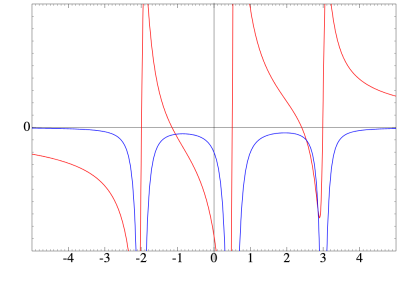
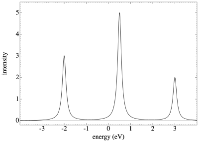
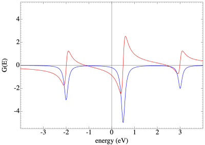
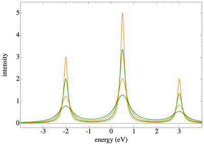
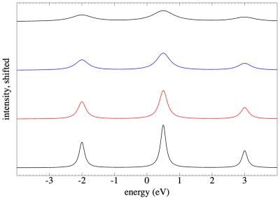
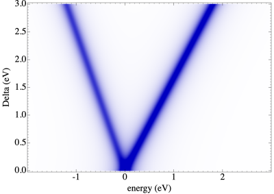
Table of contents
-